Thursday, October 8, 2015

Accessing OData from Visual Studio Online

Summary


Visual Studio Online is cloud version of TFS which we can connect using Visual Studio to retrieve projects collections and work items. The VSO does not give access to any backend database like CRM tools and exposes its data through REST API and ODATA.

Requirement : Pull project and work item collection from VSO and store the same in SQL Azure, which will be used for analysis.

Solution : Create SSIS package to connect to VSO using OData connection and pull VOS data like project , work items etc and connect to SQL Azure and store the desired data.

Prerequisite


Steps to create SSIS package

Create connection to Azure and VSO

Open SSDT and create new SQL Server Integration Service project, add a new package and go to the connection manager and right click, you will get the below window.

After clicking on new connection it takes to another window where we have to select OData.


Your connection details should look like the below for VSO.

AccountName - The collection path user is assigned to.
Password - The alternate password set in VSO.
AccountName - User account to login to VSO


Similarly create SQL Azure - Oledb connection which looks like the below one


Understand the VSO Odata service location
The VSO odata service is exposed at https://tfsodata.visualstudio.com/ which has detailed spacification of specifying the URL for different object collection.

Next is we can drag the Odata source and place in Dataflow task so the final look will be as below.


The WorkItem source details looks like shown below.


Friday, April 3, 2015

SSRS Configuration for Sharepoint

Step 1: Configuring SQL Reporting Services – Web Service URL

Simply go to Reporting Services Configuration Manager and choose Web Service URL and populate the following needed information. The fields are named properly so I guess there is no need for further explanation. What this does is that it configures the IIS for you depending on what Virtual Directory names you had declared.

Step 2: Configuring SQL Reporting Services – Create a Report Database

Same here, fields need no further explanation except for one which is Native Mode and SharePoint Integrated mode which I will explain below.
Choose create a database or if you already have one choose an existing one. For this example, we will create a new one:

Connect to the database where you want your Report Data to be stored:

Give it a Name and a Report Server Mode.
With SharePoint Integrated Mode the report RDLs are stored on SharePoint and not in the Report Database. For this instance, we will use the SharePoint Integrated Mode:

Specify the credentials that the report server will use to connect to the database.

Review your configuration.

Then wait while it's configured.

Step 3: Configuring SQL Reporting Services – Create a Report Manager URL

What this does is that it configures the IIS for you depending on what Virtual Directory names you had declared.

That’s it. At this point, your report server is configured for SharePoint Integration 2010.

Step 4: SharePoint Integration Configuration – Reporting Services Integration

Simply go to SharePoint 2010 Central Administration, then General Application Settings, then choose Reporting Services Integration.

Now populate the fields using the Web Service URL you had configured a while ago on Step 2 of this guide.

Once done, you will see the Activation State message.

Step 5: SharePoint Integration Configuration – Add a Report Server to the Integration

Now add the report server by putting the Server Name and the Server instance.

At this point it's all done, all you have to do now is try it out.

Step 6: Verify by Checking the Server and Uploading a Report

To verify if it's now integrated, go to Site Settings on your SharePoint Site, then Site Collection Features.


Check if the Report Server Integration Feature is Active, if not just click activate:

Now try to use the SQL Server Reporting Services Webpart:


Or you can also upload a report from a library.


Thursday, March 5, 2015

Step By Step Guide to Change Report Server Look and feel

CHANGE THE CONFIGURATION ENTRY IN REPORT SERVER FOLDER

·        Navigate to the report server folder which “C:\Program Files\Microsoft SQL Server \ MSRS_vv.MSSQLSERVER\Reporting Services\ReportServer”
·        Open the rsreportserver.config file and add the below entry below <Configuration>
·        <HTMLViewerStyleSheet>Pink</HTMLViewerStyleSheet> remember that Pink is will be your CSS file name which we will create in next step.
·        Save and close the file.

ADD Pink.css file in the Style folder

·        Open the Styles folder in \ReportServer and create a file named Pink.css
·        Copy the content of HTMLViewer.css to file name Pink.css.
·        Now you can modify the content of Pink.css according to your ease.
·        Suppose if you want to change the Parameter Frame color the navigate to .ParameterFrame section and modify.
e.g.

.ParametersFrame
{
/* make background ! */
background-color:burlywood;
border1px solid maroon;
width100%;
}

Accessing your newly created CSS in ReportServer

Try using the below command to access your new CSS in Report Server

http://localhost/reportserver?rc:Stylesheet=Pink


Monday, May 26, 2014

Dimensional Modelling base schema

When we think about dimensional modelling then two major and very important modeling schema comes into picture called the start schema and the snowflake schema.
So lets go into details on start and snowflake schema.

Star schema

Data Warehouse Schema Architecture - star schema
What is star schema? The star schema architecture is the simplest data warehouse schema. It is called a star schema because the diagram resembles a star, with points radiating from a center. The center of the star consists of fact table and the points of the star are the dimension tables. Usually the fact tables in a star schema are in third normal form(3NF) whereas dimensional tables are de-normalized. Despite the fact that the star schema is the simplest architecture, it is most commonly used nowadays and is recommended by Oracle.

Snowflake schema


Data Warehouse Schema Architecture - snowflake schema
What is snowflake schema? The snowflake schema architecture is a more complex variation of the star schema used in a data warehouse, because the tables which describe the dimensions are normalized. Here there can be two sets of dimensions one is called the primary dimension which is directly connected with the fact and secondary dimension which is indirectly connected with a fact through some primary dimensions.

Apart from star and snowflake we have one more schema when we try to connect two or more dimensional schema through fact and that is called as fact constellation schema.

Fact constellation schema


Data Warehouse Schema Architecture - fact constellation schema
What is fact constellation schema? For each star schema it is possible to construct fact constellation schema(for example by splitting the original star schema into more star schemes each of them describes facts on another level of dimension hierarchies). The fact constellation architecture contains multiple fact tables that share many dimension tables.

The main shortcoming of the fact constellation schema is a more complicated design because many variants for particular kinds of aggregation must be considered and selected. Moreover, dimension tables are still large.  

Dimension and Fact Types

TYPES OF DIMENSIONS

Conformed Dimension:

Conformed dimensions mean the exact same thing with every possible fact table to which they are joined.
Eg: The date dimension table connected to the sales facts is identical to the date dimension connected to the inventory facts.

Junk Dimension:

A junk dimension is a collection of random transactional codes flags and/or text attributes that are unrelated to any particular dimension. The junk dimension is simply a structure that provides a convenient place to store the junk attributes.

Eg: Assume that we have a gender dimension and marital status dimension. In the fact table we need to maintain two keys referring to these dimensions. Instead of that create a junk dimension which has all the combinations of gender and marital status (cross join gender and marital status table and create a junk table). Now we can maintain only one key in the fact table.

Degenerated Dimension:

A degenerate dimension is a dimension which is derived from the fact table and doesn't have its own dimension table.

Eg: A transactional code in a fact table.

Role-playing dimension:

Dimensions which are often used for multiple purposes within the same database are called role-playing dimensions. For example, a date dimension can be used for “date of sale", as well as "date of delivery", or "date of hire".

TYPES OF FACTS

Additive:

Additive facts are facts that can be summed up through all of the dimensions in the fact table. A sales fact is a good example for additive fact.

Semi-Additive:

Semi-additive facts are facts that can be summed up for some of the dimensions in the fact table, but not the others.
Eg: Daily balances fact can be summed up through the customers dimension but not through the time dimension.

Non-Additive:

Non-additive facts are facts that cannot be summed up for any of the dimensions present in the fact table. 
Eg: Facts which have percentages, ratios calculated.

Factless Fact Table:

In the real world, it is possible to have a fact table that contains no measures or facts. These tables are called "Factless Fact tables".

Eg: A fact table which has only product key and date key is a factless fact. There are no measures in this table. But still you can get the number products sold over a period of time.

A fact tables that contain aggregated facts are often called summary tables

SLOWLY CHANGING DIMENSION

TYPE 1

In Type 1 Slowly Changing Dimension, the new information simply overwrites the original information. In other words, no history is kept.
In our example, recall we originally have the following table:
Customer KeyNameState
1001ChristinaIllinois
After Christina moved from Illinois to California, the new information replaces the new record, and we have the following table:
Customer KeyNameState
1001ChristinaCalifornia
Advantages:
- This is the easiest way to handle the Slowly Changing Dimension problem, since there is no need to keep track of the old information.
Disadvantages:
- All history is lost. By applying this methodology, it is not possible to trace back in history. For example, in this case, the company would not be able to know that Christina lived in Illinois before.
Usage:
About 50% of the time.
When to use Type 1:
Type 1 slowly changing dimension should be used when it is not necessary for the data warehouse to keep track of historical changes.

TYPE 2

In Type 2 Slowly Changing Dimension, a new record is added to the table to represent the new information. Therefore, both the original and the new record will be present. The new record gets its own primary key.
In our example, recall we originally have the following table:
Customer KeyNameState
1001ChristinaIllinois
After Christina moved from Illinois to California, we add the new information as a new row into the table:
Customer KeyNameState
1001ChristinaIllinois
1005ChristinaCalifornia
Advantages:
- This allows us to accurately keep all historical information.
Disadvantages:
- This will cause the size of the table to grow fast. In cases where the number of rows for the table is very high to start with, storage and performance can become a concern.
- This necessarily complicates the ETL process.
Usage:
About 50% of the time.
When to use Type 2:
Type 2 slowly changing dimension should be used when it is necessary for the data warehouse to track historical changes.

TYPE 3

In Type 3 Slowly Changing Dimension, there will be two columns to indicate the particular attribute of interest, one indicating the original value, and one indicating the current value. There will also be a column that indicates when the current value becomes active.
In our example, recall we originally have the following table:
Customer KeyNameState
1001ChristinaIllinois
To accommodate Type 3 Slowly Changing Dimension, we will now have the following columns:
  • Customer Key
  • Name
  • Original State
  • Current State
  • Effective Date
After Christina moved from Illinois to California, the original information gets updated, and we have the following table (assuming the effective date of change is January 15, 2003):
Customer KeyNameOriginal StateCurrent StateEffective Date
1001ChristinaIllinoisCalifornia15-JAN-2003
Advantages:
- This does not increase the size of the table, since new information is updated.
- This allows us to keep some part of history.
Disadvantages:
- Type 3 will not be able to keep all history where an attribute is changed more than once. For example, if Christina later moves to Texas on December 15, 2003, the California information will be lost.
Usage:
Type 3 is rarely used in actual practice.
When to use Type 3:
Type III slowly changing dimension should only be used when it is necessary for the data warehouse to track historical changes, and when such changes will only occur for a finite number of time.


Friday, July 12, 2013

Using custom code in SSRS

Step by step to add custom code in SSRS

Introduction

SSRS custom code extends re-usability of certain logic in multiple places inside a report. It also helps get rid of writing lengthy calculations in many places with a function. SSRS 2005/2008R2 allows us to write custom codes in VB. If somebody is familiar with C# can choose another option called - Custom Assembly.

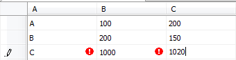
We will create a sample report with a simple Custom code which will accept two numbers and return the greater of two. So for the sample report I have a given table  Test table with three columns A,B,C


Now we will try creating a report from the source data so first we will add a new report in BIDS SSRS project. create proper data source and data set referring to the above table.
Now first we will go to Report Property and will click on the Code portion and write the below code.

After writing the code we will drag a table and will specify all the columns and will add one extra column that will return the Greater of two values. So in the last column we right click and click on the expression as below.

Now finally we add the below expression will calls the function we defined in the property section of the report.

We see that I have used Code.functionname as when we define a function the SSRS engine puts the function inside the Code class and thus we need to refer the Code before calling the function.
Now we execute the report and see the value returned is the Greater of B & C in last column.


Tuesday, July 9, 2013

Using merge join without Sort transformation

Merge join without SORT Transformation
Merge join requires the IsSorted property of the source to be set as true and the data should be ordered on the Join Key. So when we add a SORT transformation it sets the IsSorted property of the source data to true and allows the user to define a column on which we want to sort the data ( the column should be same as the join key). Now to avoid the using SORT transformation we need to set the metadata of the source properly for successful processing of the data else we get error as IsSorted property is not set to true.

We will try to join two tables Department and Employee on DeptID column without using SORT transformation in our SSIS package.

Department Table details


Employee Table details
Steps in SSIS package

  • Create a new package and drag a dataflow task.
  • Now right click on Data-flow and click on edit, the data-flow container opens.
  • First task is to create a connection to the database.   
  • Now we need to set department source, first we will drag the OLEDB Source and set connection and  table

  • Now we click on "ok" to save changes. Again we right click on department source and click on "Show Advance Editor" and go to "input output property" tab. On the "input and output property" tab we select the "OLEDB Source output" and set the IsSorted property to true as mentioned below.


  • After setting the above property we expand the "output column" and inside that we select the column (DeptID) which we will use in join and set SortKeyPosition = 1 in the properties tab as shown in below image.

  • We will repeat the same process for second source i.e the Employee table.


Once the properties set for the sources we drag the merge join transformation and set the required properties which include the sources, join key and the output columns as shown below.


Now we drag the out put of the Merge join and join to a Derieved column where in the path we also configure data viewer to check the data. Now out package Data-Flow looks like the below image.


We run the package and try to view the data which shows like below.


PowerBI monthly report refresh

How to setup monthly refresh for PowerBI ? PowerBI generally allows daily or weekly refreshes with options of selecting multiple time values...